Solution 1
| Data set | Time origin | Time scale | Event | Censoring |
|---|---|---|---|---|
| pulmonary (11 men) | Not stated; presumably diagnosis or start of treatment of the pulmonary metastasis | months | Death | None |
| iud (18 women) | First day of IUD use | weeks | Discontinuation because of menstrual bleeding | 9 censored: stopped for another reason, lost to follow-up, or reached the two-year protocol limit |
| breast (45 women) | Surgery (mastectomy) | months | Death from breast cancer | 19 censored: alive in July 1987, died of other causes, or lost to follow-up |
| myeloma (48 patients) | Diagnosis | months | Death from multiple myeloma | 12 censored at the end of the study |
| prostate (38 men) | Randomisation | months | Death from prostatic cancer | 32 censored: deaths from other causes, losses to follow-up, or administrative censoring at the end of follow-up |
| melanoma (30 patients) | Surgical removal of the tumour, then randomisation | months | Death | 20 censored: alive at the end of follow-up |
Solution 2
(The median survival time is defined in Lecture 1, slide 25; reporting survival at fixed times instead of a median is slide 24; and informative censoring is slide 11.)
n_distinct(prostate$patient)
#> [1] 38
sum(prostate$status)
#> [1] 6
The median is the smallest time at which the estimated survivor function is below 0.5. The Kaplan–Meier curve for
prostatenever crosses 0.5 and no median exists in the observed follow-up. The reported lower 95 % limit of the median is a bound: the data are compatible with a median as early as that, but the upper limit is not estimable.A sensible answer is to report survival at fixed, clinically meaningful times (for example at 36 and 60 months = 3 and 5 years), with a confidence interval and the number at risk, rather than forcing a median:
summary(surv_prostate, c(36, 60))
#> Call: survfit(formula = Surv(time, status) ~ 1, data = prostate)
#>
#>  time n.risk n.event survival std.err lower 95% CI upper 95% CI
#>    36     30       3    0.910  0.0495        0.818         1.00
#>    60     16       2    0.845  0.0639        0.729         0.98
plot(surv_prostate)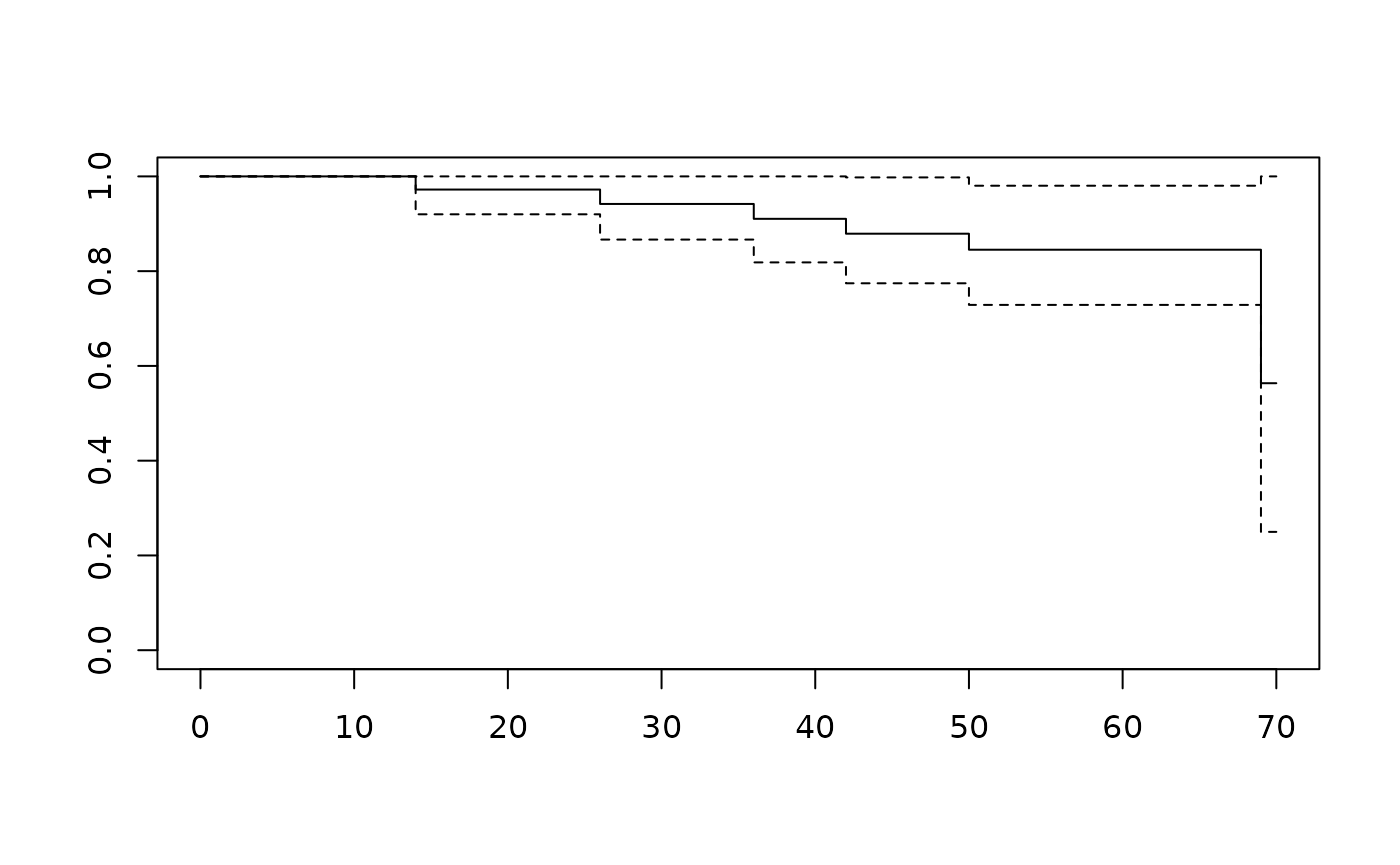
last_death <- prostate |>
  filter(status == 1) |>
  summarise(max(time)) |>
  pluck(1)
last_cens <- prostate |> filter(status == 0) |> summarise(max(time)) |> pluck(1)

prostate |> slice_max(time)
#>   patient treatment time status age  shb size index
#> 1      31         2   70      0  72 13.8    3     9
#> 2      35         2   70      0  71 13.6    2    10
The last death is at 69 months; after that the curve is flat until the last censoring at 70 months. Only 2 men are at risk at the last observed time, so the height of the curve there is determined by a very small risk set. The far right-hand tail should not be interpreted as a precise estimate of long-term survival.
It is recommended to always present a risk table with the Kaplan–Meier curve, so that the reader can see how many patients are at risk at each time point:
ggsurvfit(surv_prostate) +
  add_risktable() +
  add_confidence_interval()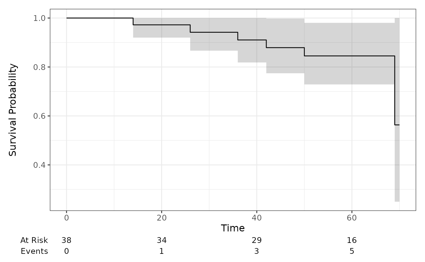
- If men who became too unwell stopped attending, their subsequent deaths would be missing and the remaining men would look healthier than they really were. The Kaplan–Meier estimate would then be biased upwards. This is dependent or informative censoring, and it violates the independent censoring assumption.
Solution 3
(Statements (b), (d), (e) and (f) revisit Lecture 1 (censoring, fixed vs random censoring, independent censoring, and study vs patient time); statement (c) is from Lecture 2 on the hazard.)
False. A patient censored at 10 months contributes to the risk set up to 10 months and is removed immediately after 10 months. She is not at risk at 12 months.
False. Informative censoring can bias the estimate in either direction. If high-risk patients leave, survival is overestimated; if low-risk patients leave, survival is underestimated.
False. The hazard is an instantaneous rate, not a probability. It is the limiting probability of an event in a short interval divided by the length of that interval, and it can be greater than 1.
True, provided the analysis time was specified in advance and the censoring is not related to prognosis. Administrative censoring at a pre-specified calendar date is the usual example of independent censoring.
True.
True.. Study time is calendar time measured from the start of the study; patient time is measured from each patient’s own time origin. If a study closes on a fixed calendar date, a patient recruited late has less patient time at closure than a patient recruited early. Administrative censoring therefore gives different patient-time censoring times, even though all patients are censored on the same calendar date. This is usually independent censoring if the closing date was pre-specified and the recruitment date is unrelated to prognosis.
Solution 4
emp_pulm
#>   time n_at_least      S_hat
#> 1   11         11 1.00000000
#> 2   13         10 0.90909091
#> 3   14          5 0.45454545
#> 4   15          3 0.27272727
#> 5   17          1 0.09090909
summary(survfit(Surv(time) ~ 1, data = pulmonary))
#> Call: survfit(formula = Surv(time) ~ 1, data = pulmonary)
#>
#>  time n.risk n.event survival std.err lower 95% CI upper 95% CI
#>    11     11       1   0.9091  0.0867        0.754        1.000
#>    13     10       5   0.4545  0.1501        0.238        0.868
#>    14      5       2   0.2727  0.1343        0.104        0.716
#>    15      3       2   0.0909  0.0867        0.014        0.589
#>    17      1       1   0.0000     NaN           NA           NA
There is a small convention issue at an event time. The empirical
definition
gives an estimate of 1.000 at 11 months, because all 11 men have a
survival time of at least 11 months. survfit() reports
0.909 at 11 months, because it lets the curve drop at the event time and
reports the value after the drop. Between event times the two
conventions agree, and at 12 months both give 0.909. The important
practical point is to say whether a reported “survival at 12 months”
includes deaths at exactly 12 months or not!
- The empirical curve is a step function that drops at the event
times, and the
ggsurvfit()version does the same but it starts from time 0 and it adds one extra segment in the end. (If you use a microscope, the difference in the convention at the event times might be visible as well.)
emp_pulm |>
  ggplot(aes(time, S_hat)) +
  geom_step(direction = "vh") +
  scale_y_continuous(limits = c(0, 1)) +
  scale_x_continuous(limits = c(0, NA)) +
  survfit2(Surv(time) ~ 1, pulmonary) |>
    ggsurvfit() +
  scale_y_continuous(limits = c(0, 1))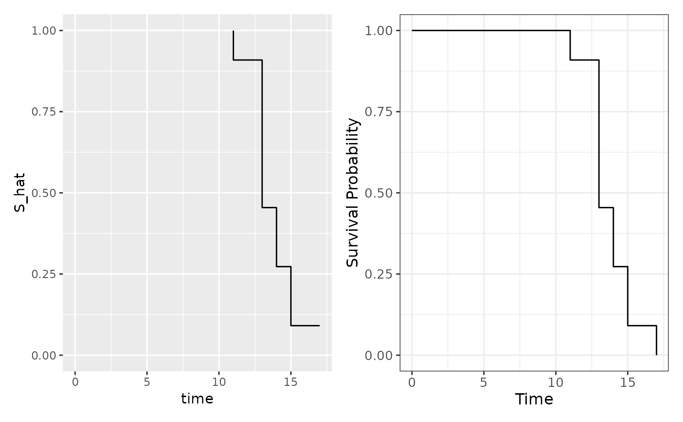
It is important to notice, however, that the similarity above would
not translate easily to the case with censoring! Consider the
prostate data set:
prostate |>
  filter(status == 1) |> # Why?
  distinct(time) |>
  arrange(time) |>
  mutate(
    n_at_least = map_int(time, \(t) sum(prostate$time >= t)),
    S_hat = n_at_least / nrow(prostate)
  ) |>
  ggplot(aes(time, S_hat)) +
  geom_step(direction = "vh") +
  scale_y_continuous(limits = c(0, 1)) +
  scale_x_continuous(limits = c(0, NA)) +
  survfit2(Surv(time, status) ~ 1, prostate) |>
    ggsurvfit() +
  scale_y_continuous(limits = c(0, 1))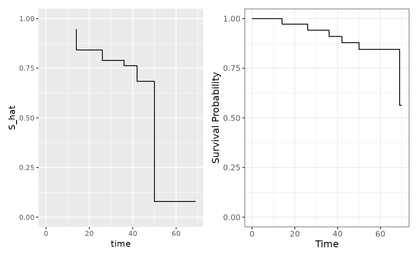
- With the empirical convention in the table, the estimate is 1.000 at 11 months and drops at 13, 14, 15, 17 months; the sizes of those drops are 0.091, 0.455, 0.182, 0.182. It is flat between 15 and 17 months because no one dies in that interval.
Solution 5
(Lecture 1, slides 18 and 25: skewed survival times and the median survival time.)
Survival times are usually right-skewed and the mean is sensitive to a few long survivors; the median is the time by which half the patients have died and is more robust. Here the mean is slightly larger than the median, which is consistent with a right tail. If the largest observation were censored, the mean would not be estimable without an assumption about the unobserved tail; treating the censored time as a death would underestimate the mean. The median can still be estimated if the curve reaches 0.5.
Solution 6
Collett discusses this in Section 2.1.2.
The censored observation should be counted after the deaths at 13 months: the risk set just before that time includes everyone still under observation at that time, including the person who is censored there. The deaths are then removed, and the censored observation is removed afterwards. If the censoring were counted before the deaths, the risk set would be too small and the estimated survival would change.
Note that the time scale here is in months. If exact dates were available, the censoring could be counted before or after the deaths depending on the exact times of the events. Then the same convention would instead be used for deaths and censoring at the same number of days since time 0.
Solution 7 (Optional)
- After 13 months, 6 of the 11 men have died, so . The binomial standard error is
This is the std.err
reported by survfit() at 13 months.
pulsurv <- survfit(Surv(time) ~ 1, data = pulmonary)
summary(pulsurv)
#> Call: survfit(formula = Surv(time) ~ 1, data = pulmonary)
#>
#>  time n.risk n.event survival std.err lower 95% CI upper 95% CI
#>    11     11       1   0.9091  0.0867        0.754        1.000
#>    13     10       5   0.4545  0.1501        0.238        0.868
#>    14      5       2   0.2727  0.1343        0.104        0.716
#>    15      3       2   0.0909  0.0867        0.014        0.589
#>    17      1       1   0.0000     NaN           NA           NA
NOTE! summary() reports the standard
error of the survival estimate, whereas broom::tidy()
reports it on the log-survival scale. If you want to compute the
standard error of the survival estimate from the
broom::tidy() output, you need to multiply the
estimate by the std.error:
broom::tidy(pulsurv) |>
  select(time, estimate, std.error) |>
  mutate(se_survival = estimate * std.error)
#> # A tibble: 5 × 4
#>    time estimate std.error se_survival
#>   <dbl>    <dbl>     <dbl>       <dbl>
#> 1    11   0.909     0.0953      0.0867
#> 2    13   0.455     0.330       0.150
#> 3    14   0.273     0.492       0.134
#> 4    15   0.0909    0.953       0.0867
#> 5 17 0 Inf NaN- At the last death time there is one person at risk and that person
dies, so
.
Greenwood’s sum contains the term
,
and
is
NaN. The estimate is zero because the only remaining person died, but that does not mean the survival probability is known with certainty; the sample is small and the tail is poorly estimated. This is one reason why the last part of a Kaplan–Meier curve is fragile.
Solution 8
(t2.2 <- tibble(event_times = sort(unique(iud$time[iud$status == 1]))) |>
  mutate(
    n_risk = map_int(event_times, \(t) sum(iud$time >= t)),
    n_event = map_int(event_times, \(t) sum(iud$time == t & iud$status == 1)),
    factor = (n_risk - n_event) / n_risk,
    estimate = cumprod(factor)
  ))
#> # A tibble: 9 × 5
#>   event_times n_risk n_event factor estimate
#>         <int>  <int>   <int>  <dbl>    <dbl>
#> 1          10     18       1  0.944    0.944
#> 2          19     15       1  0.933    0.881
#> 3          30     13       1  0.923    0.814
#> 4          36     12       1  0.917    0.746
#> 5          59      8       1  0.875    0.653
#> 6          75      7       1  0.857    0.559
#> 7          93      6       1  0.833    0.466
#> 8          97      5       1  0.8      0.373
#> 9         107      3       1  0.667    0.249
The values agree with Collett’s Table 2.2 (exept the first line where no event occured).
- The requested estimates are:
Only the last requested time point is presented in the table:
requested_times <- c(12, 24, 52, 104, 107)
t2.2 |>
  filter(event_times %in% requested_times) |>
  select(event_times, estimate)
#> # A tibble: 1 × 2
#>   event_times estimate
#>         <int>    <dbl>
#> 1         107    0.249
For the remaining ones, we need to look at the closest event time before the requested time point. For example, for 24 weeks, the closest event time is 19 weeks and the estimte does not change until week 30.
We can also use the summary() function to get the
estimates from a survfit object:
survfit(Surv(time, status) ~ 1, data = iud) |>
  summary(requested_times)
#> Call: survfit(formula = Surv(time, status) ~ 1, data = iud)
#>
#>  time n.risk n.event survival std.err lower 95% CI upper 95% CI
#>    12     17       1    0.944   0.054       0.8443        1.000
#>    24     13       1    0.881   0.079       0.7395        1.000
#>    52     10       2    0.746   0.111       0.5577        0.998
#>   104      4       4    0.373   0.143       0.1759        0.791
#>   107      3       1    0.249   0.139       0.0829        0.745
Note that n.risk is updated to reflect the number of
women at risk at the requested time points (but this does not affect the
survival estimate).
Solution 9
- The largest observed time is for:
slice_max(iud, time)
#>   time status
#> 1  107      1
#> 2  107      0
#> 3  107      0
The Kaplan–Meier estimate stays constant from week 97, until just before week 107. It is not defined after 107 weeks, because there is no one left at risk after the event and the censorings at week 107.
If all observations at week 107 had been censored, there would be no event, so the estimate would remain from week 97, and it would still be undefined after week 107. If the only observation at week 107 had been an event with no other person at risk at that time, the factor would be and the curve would drop to zero at week 107.
Beyond the largest observed time there is no information about the event rate; no one is under observation. Continuing the curve flat would assume that no events occur after the end of follow-up, which is an extra assumption, not a result of the data. The curve therefore stops at the last observed time.
Solution 10
ggplot(haz, aes(t, h)) + geom_step()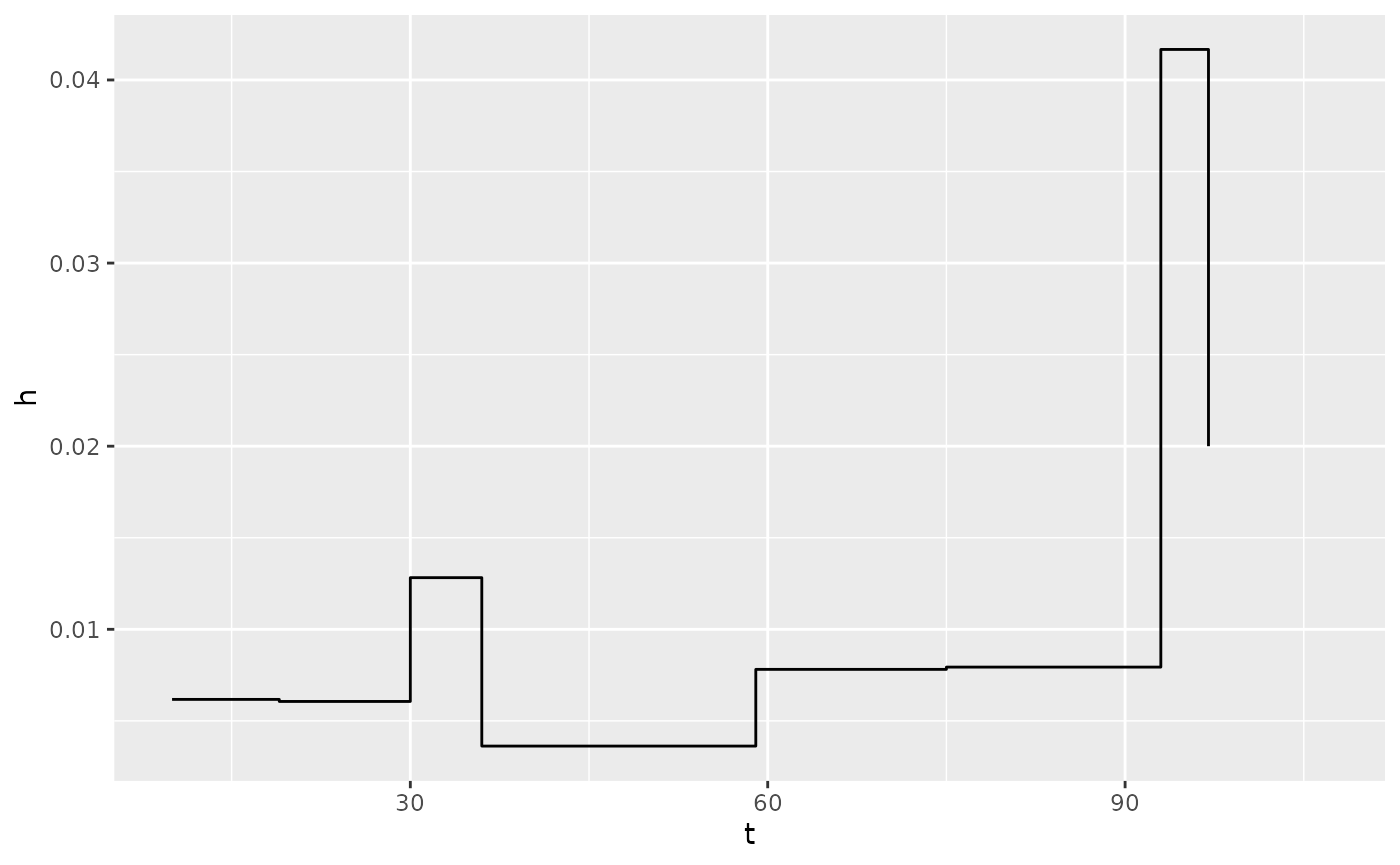
A similar graph may be produced using the muhaz package, but its kphaz.fit() function uses the event and risk set at the end of each interval and places the estimate at the midpoint. Hence, the results are slightly different from the above, but the overall shape is similar.
library(muhaz)
haz2 <- with(iud, kphaz.fit(time, status, method = "product-limit"))
kphaz.plot(haz2)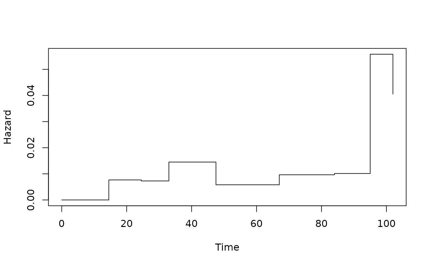
A single death among a small risk set over a short interval produces a large and unstable rate; a single death among a large risk set over a long interval produces a small one.
- The cumulative hazard and the survivor function are cumulative summaries: they use all the information up to time and are much more stable than a sequence of pointwise hazard estimates. A raw hazard plot is useful for exploring shape, but it is not a precise summary, especially in small samples.
Solution 11
The naive estimate:
naive_events <- filter(iud, status == 1 & time <= 104) |> nrow()
1 - naive_events / nrow(iud)
#> [1] 0.5555556
Kaplan–Meier estimate:
survfit(Surv(time, status) ~ 1, data = iud) |>
  summary(104) |>
  _$surv
#> [1] 0.3729345
The naive estimate is too high by about 13 percentage points.
The naive calculation treats the 9 censored women as if they had not discontinued during the full 104 weeks. In fact, they were only followed until their censoring time, and some of them would have discontinued later. Ignoring that incomplete follow-up inflates the estimated survival.
The problem would be worse with 80 % censoring: more of the denominator would consist of women with incomplete follow-up treated as if they had completed the study. The bias would generally be larger.
“The estimated probability that a woman is still using the IUD at 104 weeks (2 years) is 0.37, assuming that censoring is non-informative.” Or: “About 37 % of women are estimated to remain free of discontinuation due to bleeding at 2 years.”
Solution 12
(This is Lecture 2 material: the hazard is the instantaneous event rate at time — the probability of an event in a short interval given no event before , divided by the interval length — and the cumulative hazard sums it up.)
# Kaplan–Meier
km <- survfit(
  Surv(time, status) ~ 1,
  data = sta310r::myeloma,
  stype = 1, # "direct" = "Kaplan-Meier" = "product-limit"
  ctype = 1
)

# exp(-Nelson–Aalen)
na_surv <- survfit(
  Surv(time, status) ~ 1,
  data = sta310r::myeloma,
  stype = 2, # exp(cumulative hazard) where cumhaz = Nelson–Aalen from ctype = 1
  ctype = 1
)

bind_rows(km = broom::tidy(km), na = broom::tidy(na_surv), .id = "estimator") |>
  ggplot(aes(time, estimate, color = estimator)) +
  geom_step(direction = "hv")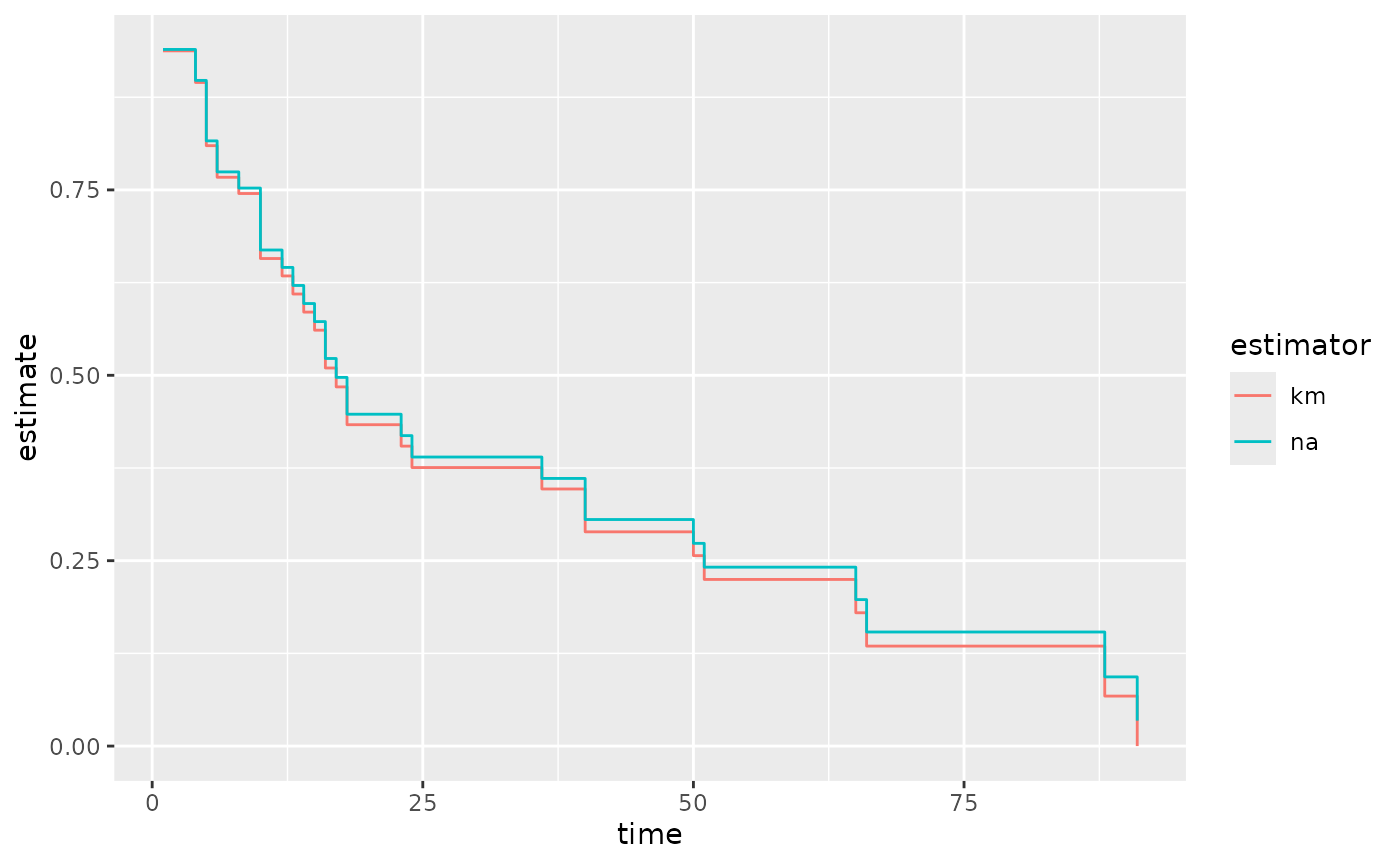
The Nelson–Aalen survivor estimate is larger than the Kaplan–Meier estimate!
- The slope of the cumulative hazard curve is the hazard: a steeper slope means a higher event rate.
ggsurvfit(km, type = "cumhaz") +
  ggsurvfit(na_surv, type = "cumhaz")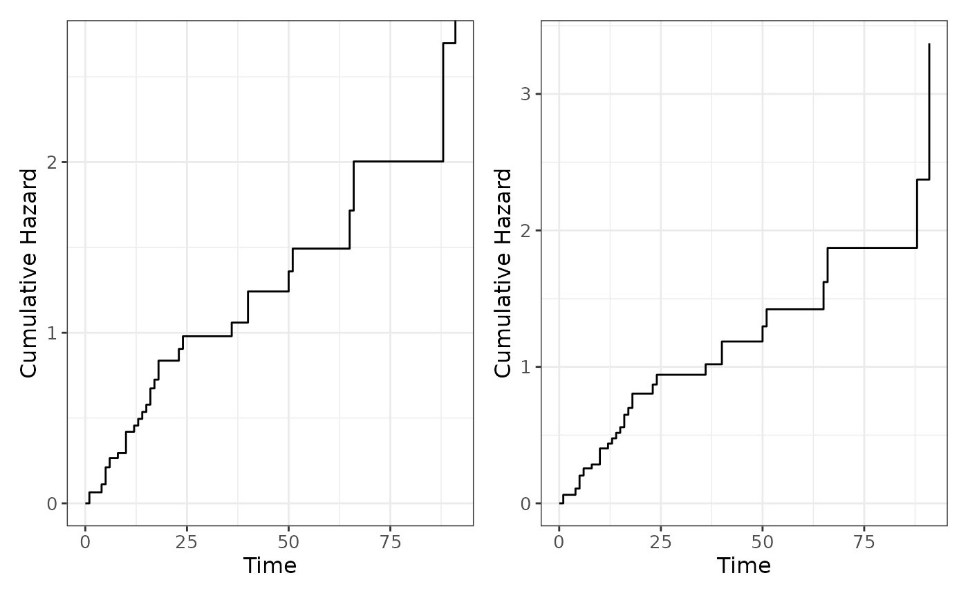
- The differences at month 24 in cumulative hazard and survival are
summary(na_surv, 24)$cumhaz - summary(km, 24)$cumhaz
#> [1] 0
summary(na_surv, 24)$surv - summary(km, 24)$surv
#> [1] 0.01419884
This is small compared to the SEs:
The difference between the estimators is therefore not practically important compared with the statistical uncertainty.
ggsurvfit(km, title = "hej") +
  add_confidence_interval() +
  ggsurvfit(na_surv) +
  add_confidence_interval()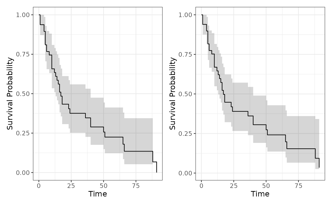
Solution 13
survfit2(Surv(time, status) ~ stain, data = breast) |>
  ggsurvfit() +
  add_confidence_interval() +
  add_quantile(y_value = 0.5) +
  add_risktable() +
  add_pvalue() # vNot asked for but useful to add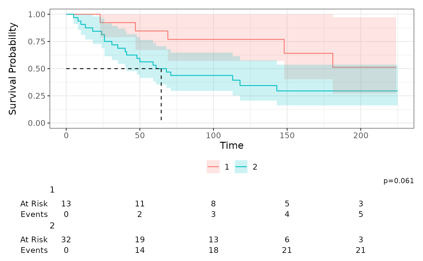
km_breast <- survfit(Surv(time, status) ~ stain, data = breast)

tbl_survfit(
  km_breast,
  times = c(24, 60, 120),
  label_header = "**Time {time} months**"
)| Characteristic | Time 24 months | Time 60 months | Time 120 months |
|---|---|---|---|
| stain | |||
| 1 | 92% (79%, 100%) | 85% (67%, 100%) | 77% (57%, 100%) |
| 2 | 81% (69%, 96%) | 53% (38%, 74%) | 34% (21%, 58%) |
summary(km_breast, times = c(24, 60, 120), extend = TRUE)
#> Call: survfit(formula = Surv(time, status) ~ stain, data = breast)
#>
#>                 stain=1
#>  time n.risk n.event survival std.err lower 95% CI upper 95% CI
#>    24     12       1    0.923  0.0739        0.789            1
#>    60     11       1    0.846  0.1001        0.671            1
#>   120      6       1    0.769  0.1169        0.571            1
#>
#>                 stain=2
#>  time n.risk n.event survival std.err lower 95% CI upper 95% CI
#>    24     27       6    0.812  0.0690        0.688        0.960
#>    60     17       9    0.531  0.0882        0.384        0.736
#>   120      7       5    0.345  0.0906        0.206        0.577
Women with HPA-negative tumours have better survival at every time point. The direction is consistent with the biological hypothesis that positive staining marks a tumour with metastatic potential, but the study is small and observational.
The median is not estimable in the negative group, although its lower 95 % limit is.
km_breast
#> Call: survfit(formula = Surv(time, status) ~ stain, data = breast)
#>
#>          n events median 0.95LCL 0.95UCL
#> stain=1 13      5     NA     148      NA
#> stain=2 32     21   64.5      41      NA
The estimated curves do not cross: the negative group is above the positive group throughout. This is the pattern in which the log-rank test is the natural default (Collett, Section 2.6.5). The Wilcoxon and Peto–Peto tests are alternatives that put more weight on early differences; they are more useful when the curves cross or when the early difference is the hypothesis of interest.
The log-rank p-value was already added to the figure above. Alternatively:
survdiff(Surv(time, status) ~ stain, breast, rho = 0) # log-rank
#> Call:
#> survdiff(formula = Surv(time, status) ~ stain, data = breast,
#>     rho = 0)
#>
#>          N Observed Expected (O-E)^2/E (O-E)^2/V
#> stain=1 13        5     9.57      2.18      3.51
#> stain=2 32       21    16.43      1.27      3.51
#>
#>  Chisq= 3.5  on 1 degrees of freedom, p= 0.06
survdiff(Surv(time, status) ~ stain, breast, rho = 1) # Peto & Peto
#> Call:
#> survdiff(formula = Surv(time, status) ~ stain, data = breast,
#>     rho = 1)
#>
#>          N Observed Expected (O-E)^2/E (O-E)^2/V
#> stain=1 13      3.0      6.6      1.97      4.11
#> stain=2 32     15.7     12.1      1.08      4.11
#>
#>  Chisq= 4.1  on 1 degrees of freedom, p= 0.04
Solution 14
bcg <- melanoma |> filter(treatment == 1)- The null hypothesis is that the survival distributions are the same in the three age groups among patients treated with BCG. There are 3 groups, so the test has 2 degrees of freedom.
(x <- survdiff(Surv(time, status) ~ age, data = bcg))
#> Call:
#> survdiff(formula = Surv(time, status) ~ age, data = bcg)
#>
#>       N Observed Expected (O-E)^2/E (O-E)^2/V
#> age=1 6        2    3.187    0.4422    1.2449
#> age=2 3        1    1.195    0.0318    0.0419
#> age=3 2        2    0.618    3.0912    3.6953
#>
#>  Chisq= 3.7  on 2 degrees of freedom, p= 0.2
The test statistic is 3.7389012, p = 0.1542084. The oldest group (age = 3) contributes most (biggest difference between observed and expected).
table(bcg$age)
#>
#> 1 2 3
#> 6 3 2
The three age groups are small, so the test has very little power. A non-significant result is not evidence that the groups are the same; it means that these data are compatible with no difference. The small numbers also make the asymptotic chi-square approximation questionable.
Solution 15
bind_rows(
  unstratified = survdiff(Surv(time, status) ~ treatment, melanoma) |>
    broom::glance(),
  stratified = survdiff(
    Surv(time, status) ~ treatment + strata(age),
    data = melanoma
  ) |>
    broom::glance(),
  .id = "analysis"
) |>
knitr::kable(digits = 3)| analysis | statistic | df | p.value |
|---|---|---|---|
| unstratified | 0.756 | 1 | 0.385 |
| stratified | 0.688 | 1 | 0.407 |
The stratified test compares the treatments within each age stratum and combines the observed-minus-expected differences and their variances across strata. It estimates a common treatment effect while allowing each age group to have its own baseline hazard. It assumes that the treatment effect is the same in each age stratum (no treatment-by-age interaction) and that the strata are comparable in the sense required by the test.
The age distribution is fairly balanced between the treatment groups:
gtsummary::tbl_summary(melanoma, treatment, include = age) |>
gtsummary::add_difference(~"smd")| Characteristic |
1 N = 111 |
2 N = 191 |
Difference | 95% CI | p-value |
|---|---|---|---|---|---|
| age | |||||
| 1 | 6 (55%) | 9 (47%) | |||
| 2 | 3 (27%) | 7 (37%) | |||
| 3 | 2 (18%) | 3 (16%) | |||
| 1 n (%) | |||||
| Abbreviation: CI = Confidence Interval | |||||
Age does not appear to be a strong confounder here. Stratification removes a small amount of age imbalance but does not change the conclusion.
- Stratification can change the conclusion when age (or another stratifying factor) is strongly prognostic and the treatment groups differ substantially in its distribution. For example, if older patients were much more likely to receive one treatment and older age strongly increased mortality, the unstratified test could attribute the age effect to treatment. A stratified test would remove that confounding. If the treatment effect itself differs across strata, a common-effect stratified test may be misleading, and stratum-specific estimates or an interaction test would be needed.