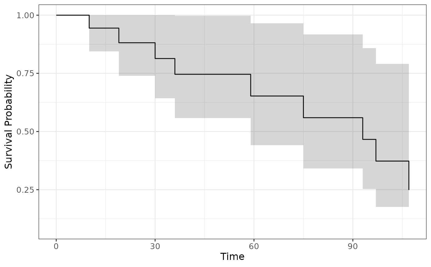
Number of weeks from the start of use of a Multiload 250 intrauterine device until discontinuation because of menstrual bleeding problems, for 18 women (Collett, 2023, Example 1.1). The data come from a World Health Organization study of contraceptive methods.
Format
A data frame with 18 rows and 2 variables:
- time
Time from first use of the IUD to discontinuation, in weeks.
- status
Event indicator: 1 = discontinuation due to menstrual bleeding problems, 0 = right-censored.
Source
Collett, D. (2023) Modelling Survival Data in Medical Research, 4th ed. Chapman & Hall/CRC, Example 1.1 (Table 1.1). Data from the World Health Organization (1987).
Details
The time origin is the first day of IUD use and the endpoint is discontinuation because of bleeding problems. Women who stopped using the device for other reasons (desire for pregnancy, no further need of contraception, lost to follow-up) contribute censored observations, as do three women whose follow-up extended beyond the two-year study protocol. There are 9 events and 9 censored times among the 18 women, three of the censored times being greater than 104 weeks.
The data are small enough to illustrate the product-limit estimator by hand. In the book they are used for the Kaplan-Meier estimate and the median (Examples 2.3-2.10), for exponential, Weibull and log-logistic parametric models (Examples 5.1-5.4) and for Bayesian analyses (Examples 16.1-16.3).
Aliases
The data set is available under the aliases d1.1, d2.3, d2.4, d2.5,
d2.7, d2.8, d2.9, d2.10, d5.1, d5.2, d5.3, d5.4, d16.1,
d16.2, d16.3; dX.Y is the alias for the data set used in Example X.Y
of Collett (2023). See dataset_by_exercise for the complete index.
Examples
# Collett (2023), Chapter 17 style -----------------------------------
# Example 1.1: times to discontinuation of an IUD
survival::survfit(survival::Surv(time, status) ~ 1, data = iud)
#> Call: survfit(formula = survival::Surv(time, status) ~ 1, data = iud)
#>
#> n events median 0.95LCL 0.95UCL
#> [1,] 18 9 93 59 NA
# Examples 2.3-2.5 and 2.7-2.10: product-limit estimate and the median
km_iud <- survival::survfit(survival::Surv(time, status) ~ 1, data = iud)
summary(km_iud, times = c(12, 24, 48))
#> Call: survfit(formula = survival::Surv(time, status) ~ 1, data = iud)
#>
#> time n.risk n.event survival std.err lower 95% CI upper 95% CI
#> 12 17 1 0.944 0.054 0.844 1.000
#> 24 13 1 0.881 0.079 0.739 1.000
#> 48 10 2 0.746 0.111 0.558 0.998
quantile(km_iud, probs = c(0.25, 0.5, 0.75))
#> $quantile
#> 25 50 75
#> 36 93 107
#>
#> $lower
#> 25 50 75
#> 19 59 97
#>
#> $upper
#> 25 50 75
#> 107 NA NA
#>
# Examples 5.1-5.4: exponential, Weibull and log-logistic models
survival::survreg(survival::Surv(time, status) ~ 1, data = iud, dist = "exponential")
#> Call:
#> survival::survreg(formula = survival::Surv(time, status) ~ 1,
#> data = iud, dist = "exponential")
#>
#> Coefficients:
#> (Intercept)
#> 4.755504
#>
#> Scale fixed at 1
#>
#> Loglik(model)= -51.8 Loglik(intercept only)= -51.8
#> n= 18
survival::survreg(survival::Surv(time, status) ~ 1, data = iud, dist = "weibull")
#> Call:
#> survival::survreg(formula = survival::Surv(time, status) ~ 1,
#> data = iud, dist = "weibull")
#>
#> Coefficients:
#> (Intercept)
#> 4.591518
#>
#> Scale= 0.5965153
#>
#> Loglik(model)= -50.4 Loglik(intercept only)= -50.4
#> n= 18
survival::survreg(survival::Surv(time, status) ~ 1, data = iud, dist = "loglogistic")
#> Call:
#> survival::survreg(formula = survival::Surv(time, status) ~ 1,
#> data = iud, dist = "loglogistic")
#>
#> Coefficients:
#> (Intercept)
#> 4.373277
#>
#> Scale= 0.5164638
#>
#> Loglik(model)= -50.9 Loglik(intercept only)= -50.9
#> n= 18
# Examples 16.1-16.3: conjugate gamma posterior for the exponential rate
# (a vague Gamma(0.001, 0.001) prior, as in the book)
a1 <- 0.001 + sum(iud$status)
b1 <- 0.001 + sum(iud$time)
c(mean = a1 / b1, stats::qgamma(c(0.025, 0.975), a1, b1))
#> mean
#> 0.008605154 0.003935029 0.015071228
# For a non-conjugate model Chapter 17 uses rstanarm::stan_surv().
# Modern tools --------------------------------------------------------
if (requireNamespace("ggsurvfit", quietly = TRUE)) {
ggsurvfit::survfit2(survival::Surv(time, status) ~ 1, data = iud) |>
ggsurvfit::ggsurvfit() +
ggsurvfit::add_confidence_interval()
}
 if (requireNamespace("flexsurv", quietly = TRUE)) {
flexsurv::flexsurvreg(survival::Surv(time, status) ~ 1, data = iud, dist = "weibull")
}
#> Call:
#> flexsurv::flexsurvreg(formula = survival::Surv(time, status) ~
#> 1, data = iud, dist = "weibull")
#>
#> Estimates:
#> est L95% U95% se
#> shape 1.676 0.979 2.872 0.460
#> scale 98.644 66.086 147.242 20.160
#>
#> N = 18, Events: 9, Censored: 9
#> Total time at risk: 1046
#> Log-likelihood = -50.35232, df = 2
#> AIC = 104.7046
#>