Survival times and causes of death for 181 irradiated mice, reared in a standard or a germ-free environment (Collett, 2023, Example 12.7).
Format
A data frame with 181 rows and 3 variables:
- environment
Rearing environment: 1 = standard, 2 = germ-free.
- causeofdeath
Cause of death: 1 = thymic lymphoma, 2 = reticulum cell sarcoma, 3 = other causes.
- time
Survival time in days.
Source
Collett, D. (2023) Modelling Survival Data in Medical Research, 4th ed. Chapman & Hall/CRC, Example 12.7 (Table 12.7). Data first described by Hoel (1972).
Details
The mice were RFM strain males, a strain susceptible to tumour development after exposure to ionising radiation, and were given 300 rads at five or six weeks of age. An autopsy established the cause of death for every mouse. There is no censoring. There are 99 mice in the standard environment (22 deaths from thymic lymphoma, 38 from reticulum cell sarcoma and 39 from other causes) and 82 in the germ-free environment (29, 15 and 38).
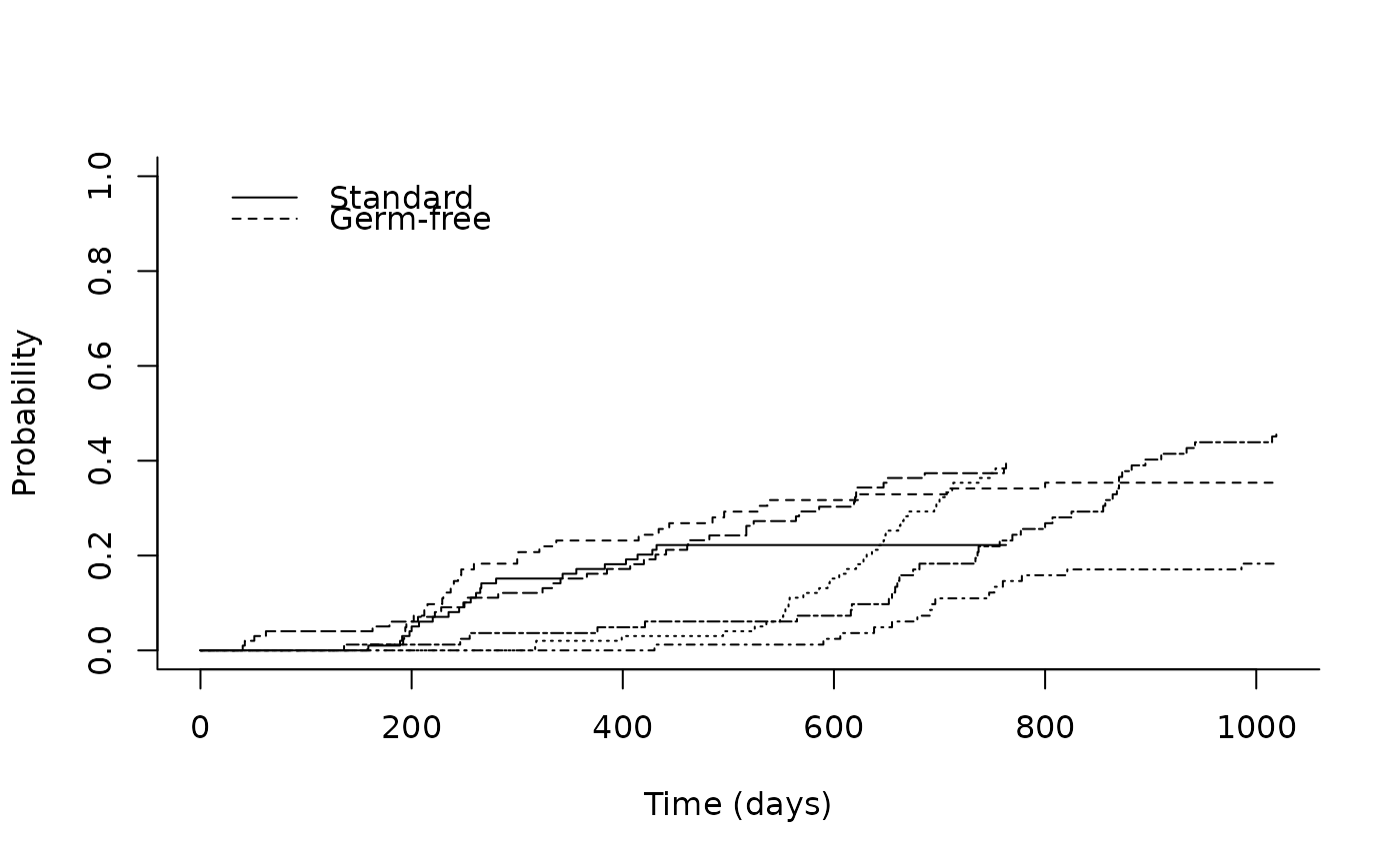
The data illustrate estimation of the cumulative incidence function for each cause and cause-specific Cox regression (Example 12.7).
Aliases
The data set is available under the alias d12.7; dX.Y is the alias for
the data set used in Example X.Y of Collett (2023). See
dataset_by_exercise for the complete index.
Examples
# Collett (2023), Chapter 17 style -----------------------------------
# Example 12.7: three competing causes of death
# (1 = thymic lymphoma, 2 = reticulum cell sarcoma, 3 = other causes)
ci_mice <- cmprsk::cuminc(mice$time, mice$causeofdeath, mice$environment)
plot(ci_mice, curvlab = c("Standard", "Germ-free"), xlab = "Time (days)")
 # Modern tools --------------------------------------------------------
if (requireNamespace("tidycmprsk", quietly = TRUE)) {
tidycmprsk::cuminc(
survival::Surv(time, factor(causeofdeath)) ~ environment,
data = mice
)
}
#>
#> ── cuminc() ────────────────────────────────────────────────────────────────────
#>
#> • Failure type "2"
#> strata time n.risk estimate std.error 95% CI
#> 1 200 89 0.000 0.000 NA, NA
#> 1 400 61 0.037 0.021 0.010, 0.095
#> 1 600 32 0.200 0.047 0.118, 0.298
#> 1 800 0 0.513 0.059 0.393, 0.620
#> 1 1,000 0 0.513 0.059 0.393, 0.620
#> 2 200 76 0.000 0.000 NA, NA
#> 2 400 59 0.000 0.000 NA, NA
#> 2 600 48 0.034 0.024 0.006, 0.107
#> 2 800 20 0.241 0.059 0.136, 0.363
#> 2 1,000 2 0.282 0.064 0.165, 0.410
#>
#> • Failure type "3"
#> strata time n.risk estimate std.error 95% CI
#> 1 200 89 0.061 0.024 0.025, 0.120
#> 1 400 61 0.189 0.042 0.115, 0.278
#> 1 600 32 0.365 0.055 0.260, 0.470
#> 1 800 0 0.487 0.060 0.366, 0.598
#> 1 1,000 0 0.487 0.060 0.366, 0.598
#> 2 200 76 0.012 0.012 0.001, 0.059
#> 2 400 59 0.057 0.028 0.018, 0.130
#> 2 600 48 0.092 0.036 0.037, 0.178
#> 2 800 20 0.393 0.067 0.263, 0.521
#> 2 1,000 2 0.678 0.067 0.527, 0.789
#>
#> • Tests
#> outcome statistic df p.value
#> 2 13.1 1.00 <0.001
#> 3 5.91 1.00 0.015