Pulmonary metastasis in patients with osteosarcoma

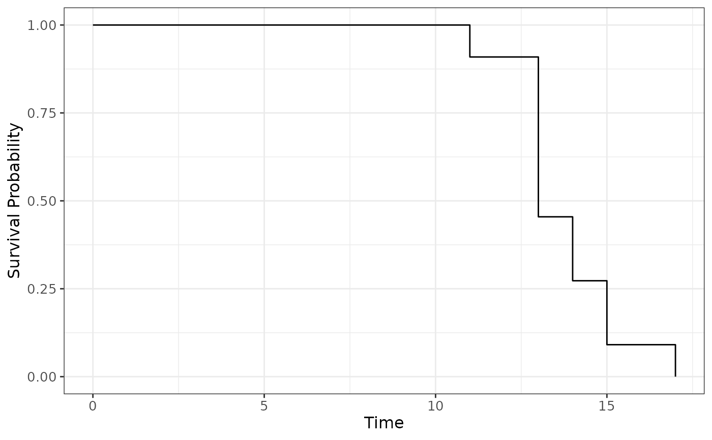
Survival times, in months, of eleven male patients with pulmonary metastasis arising from osteosarcoma (Collett, 2023, Example 2.1).

Usage

pulmonary

Format

A data frame with 11 rows and 1 variable:

time

Survival time in months.

Source

Collett, D. (2023) Modelling Survival Data in Medical Research, 4th ed. Chapman & Hall/CRC, Example 2.1. Data from Burdette and Gehan (1970).

Details

There is no censoring in these data and all survival times are distinct, so the survivor function can be estimated directly from the observed proportions surviving. The estimated values of S(t) at 11, 13, 14, 15 and 17 months are 1.000, 0.909, 0.455, 0.273 and 0.091, and S(t) is zero after 17 months. The example is used in the book to introduce the empirical survivor function before censoring is considered.

Aliases

The data set is available under the alias d2.1; dX.Y is the alias for the data set used in Example X.Y of Collett (2023). See dataset_by_exercise for the complete index.

Examples

# Collett (2023), Chapter 17 style -----------------------------------
# Example 2.1: no censoring, so Surv() needs only the time
survival::survfit(survival::Surv(time) ~ 1, data = pulmonary)
#> Call: survfit(formula = survival::Surv(time) ~ 1, data = pulmonary)
#> 
#>       n events median 0.95LCL 0.95UCL
#> [1,] 11     11     13      13      NA

# Modern tools --------------------------------------------------------
if (requireNamespace("ggsurvfit", quietly = TRUE)) {
  ggsurvfit::survfit2(survival::Surv(time) ~ 1, data = pulmonary) |>
    ggsurvfit::ggsurvfit()
}